从零构建大模型-LoRA微调

《从零构建大模型》

 [美]塞巴斯蒂安·拉施卡

书中资料 https://github.com/rasbt/LLMs-from-scratch

附录E 使用LoRA进行参数高效微调

LoRA(低秩自适应)是应用最广泛的参数高效微调技术之一。

LoRA简介

LoRA是一种通过仅调整模型权重参数的一小部分,使预训练模型更好地适应特定且通常较小的数据集的技术。“低秩”指的是将模型调整限制在总权重参数空间的较小维度子空间,从而有效捕获训练过程中对权重参数变化影响最大的方向。

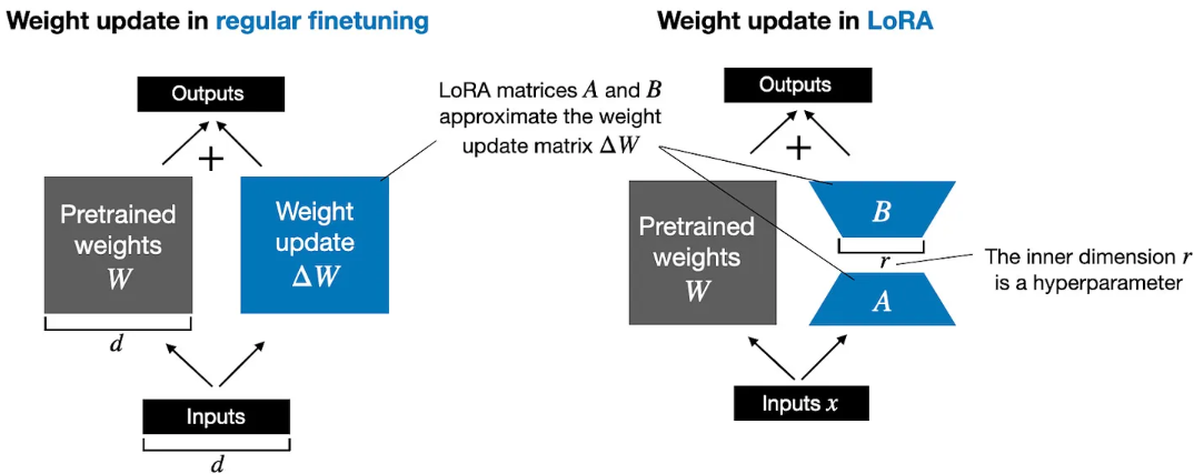
对于模型的某一个层对应的巨大的权重矩阵$W$,在模型训练反向传播的过程中,通过计算最小化损失函数得到的更新权重参数矩阵$\Delta W$,最终更新后的权重为:

$$W_{\text{updated}} = W + \Delta W$$

Hu et al. 提出的LoRA提供了一个更高效的计算权重更新 $\Delta W$ 方法,通过两个小的多子矩阵相乘得到$\Delta W \approx AB$,对于最终的权重就变为:

$$W_{\text{updated}} = W + AB$$

由于矩阵乘法的分配律,它允许我们将原始权重与更新后的权重分开,而不是将它们组合在一起,即 $$x (W+\Delta W) = x W + x \Delta W$$

因此对于LoRA方法也就有:$$x (W+A B) = x W + x A B$$,可以从下图看到LoRA和全量训练的差异,同时将LoRA权重矩阵与原始模型权重分开的能力使LoRA在实践中更加有用。从而允许预训练的模型权重保持不变,并且在使用模型时可以动态地应用LoRA矩阵。这样模型定制变得更加灵活,无须存储多个完整版本的大语言模型。这降低了存储需求并提高了可扩展性,因为在为每个特定客户或应用程序进行定制时,只需调整和保存较小的LoRA矩阵即可。

lora_basic
lora_basic

准备数据集

数据准备和第6章完全相同,将数据集分成3部分:70%用于训练,10%用于验证,20%用于测试。

1
2
3
4
5
6
7
8
9
10
11
12
13
14
15
16
17
18
19
20
21
22
23
24
25
26
27
28
29
30
31
32
33
34
import pandas as pd
def create_balanced_dataset():
# 需要删除原始文件中5082行内容开头的",这一行只有一个"会导致直到下一个"行的内容都被当作一条短信
df = pd.read_csv(".\\sms\\SMSSpamCollection.tsv", sep="\t", header=None, names=["Label", "Text"])
print(df) # [5574 rows x 2 columns]
print(df["Label"].value_counts()) # ham 4827 spam 747
# 统计垃圾信息的条数 747
num_spam = df[df["Label"] == "spam"].shape[0]

# 对正常信息数据随机采样,使它的条数和垃圾信息的条数相同
ham_subset = df[df["Label"] == "ham"].sample(num_spam, random_state=123)

# 把两个数据集合并
balanced_df = pd.concat([ham_subset, df[df["Label"] == "spam"]])
# 把标签映射成数字0和1
balanced_df["Label"] = balanced_df["Label"].map({"ham": 0, "spam": 1})

train_frac = 0.7 # 训练集的比例为0.7
validation_frac = 0.1 # 验证集的比例为0.1
# 先打乱所有的数据集 两个标签各747条,一共1494条数据
balanced_df = balanced_df.sample(frac=1, random_state=123).reset_index(drop=True)

# 按训练集和验证集的比例把数据分组
train_end = int(len(balanced_df) * train_frac)
validation_end = train_end + int(len(balanced_df) * validation_frac)

# Split the DataFrame
train_df = balanced_df[:train_end]
validation_df = balanced_df[train_end:validation_end]
test_df = balanced_df[validation_end:]
# 保存数据,不用每次都准备
train_df.to_csv("train.csv", index=None)
validation_df.to_csv("validation.csv", index=None)
test_df.to_csv("test.csv", index=None)

三个数据集分别存储到一个文件中,以后可以复用。

创建数据加载器
1
2
3
4
5
6
7
8
9
10
11
12
13
14
15
16
17
18
19
20
21
22
23
24
25
26
27
28
29
30
31
32
33
34
35
36
37
38
39
40
41
42
43
44
45
46
47
48
49
50
51
52
53
54
55
56
57
58
59
60
61
62
63
64
65
66
67
68
69
70
71
72
73
74
75
76
77
78
79
80
81
82
83
84
85
86
87
88
89
from torch.utils.data import Dataset
class SpamDataset(Dataset):
def __init__(self, csv_file, tokenizer, max_length=None, pad_token_id=50256):
self.data = pd.read_csv(csv_file)

# 处理每一行短信内容数据为词元id,这也是输入数据
self.encoded_texts = [
tokenizer.encode(text) for text in self.data["Text"]
]

if max_length is None:
self.max_length = self._longest_encoded_length()
else:
self.max_length = max_length
# 如果文版长度大于输入参数的长度,把文本长度截断到最大长度
self.encoded_texts = [
encoded_text[:self.max_length]
for encoded_text in self.encoded_texts
]

# 长度不够的文本使用pad_token_id进行填充
self.encoded_texts = [
encoded_text + [pad_token_id] * (self.max_length - len(encoded_text))
for encoded_text in self.encoded_texts
]

def __getitem__(self, index):
encoded = self.encoded_texts[index]
# 目标数据是每一行对应的标签0或1
label = self.data.iloc[index]["Label"]
return (
torch.tensor(encoded, dtype=torch.long),
torch.tensor(label, dtype=torch.long)
)

def __len__(self):
return len(self.data)

# 找出数据集中最长的文本长度
def _longest_encoded_length(self):
return max(len(encoded_text) for encoded_text in self.encoded_texts)

def create_sms_data_loaders():
tokenizer = tiktoken.get_encoding("gpt2")
print(tokenizer.encode("<|endoftext|>", allowed_special={"<|endoftext|>"})) # [50256]

num_workers = 0
batch_size = 8
torch.manual_seed(123)

train_dataset = SpamDataset(
csv_file="train.csv",
max_length=None,
tokenizer=tokenizer
)

val_dataset = SpamDataset(
csv_file="validation.csv",
max_length=train_dataset.max_length, # 验证集和测试集的长度和训练集一样
tokenizer=tokenizer
)

test_dataset = SpamDataset(
csv_file="test.csv",
max_length=train_dataset.max_length, # 验证集和测试集的长度和训练集一样
tokenizer=tokenizer
)

train_loader = DataLoader(
dataset=train_dataset,
batch_size=batch_size,
shuffle=True,
num_workers=num_workers,
drop_last=True,
)

val_loader = DataLoader(
dataset=val_dataset,
batch_size=batch_size,
num_workers=num_workers,
drop_last=False,
)

test_loader = DataLoader(
dataset=test_dataset,
batch_size=batch_size,
num_workers=num_workers,
drop_last=False,
)

加载预训练模型

第5章一样加载预训练好的GPT2模型

1
2
3
4
5
6
7
8
9
10
11
12
13
14
BASE_CONFIG = {
"vocab_size": 50257, # Vocabulary size
"emb_dim": 768,
"n_layers": 12,
"n_heads": 12,
"context_length": 1024, # Context length
"drop_rate": 0.0, # Dropout rate
"qkv_bias": True # Query-key-value bias
}

settings, params = load_gpt_models(model_size='124M', models_dir="gpt2")
model = GPTModel(BASE_CONFIG)
load_weights_into_gpt(model, params)
model.eval()
设置模型进行分类

把模型的输出层替换为2维输出线性层,并输出训练前的准确率

1
2
3
4
5
6
7
8
9
10
11
12
13
14
15
16
torch.manual_seed(123)
# set DISABLE_ADDMM_CUDA_LT=1
device = torch.device("cuda" if torch.cuda.is_available() else "cpu")
num_classes = 2 # 0表示非垃圾短信,1表示垃圾短信
# 重新定义输出层
model.out_head = torch.nn.Linear(in_features=768, out_features=num_classes).to(device)
model.to(device)

torch.manual_seed(123)
train_accuracy = calc_accuracy_loader(train_loader, model, device, num_batches=10)
val_accuracy = calc_accuracy_loader(val_loader, model, device, num_batches=10)
test_accuracy = calc_accuracy_loader(test_loader, model, device, num_batches=10)

print(f"Training accuracy: {train_accuracy*100:.2f}%") # 46.25%
print(f"Validation accuracy: {val_accuracy*100:.2f}%") # 45.00%
print(f"Test accuracy: {test_accuracy*100:.2f}%") # 48.75%

替换模型中的线性层为LoRA

定义LoRA层

它创建了矩阵$A$ 和$B$,并设置两个超参数alpha缩放因子和rank(($r$))。该层可以接受输入并计算相应的输出。

rank作为A和B两个矩阵内部的维度,大小决定了参数总数量。例如之前权重矩阵的大小为[1024,768],它的值的个数1024*768=786432,把它用矩阵乘法分拆后为A[1024,8]乘B[8,768],其中A和B总共的参数个数(两个矩阵中值的个数)为1024*8+8*768=14336 ,Lora使用的参数数量是原来的0.018,大幅缩小了参数数量。如果rank值增加,参数量也会相应增大。

由于矩阵B的初始值被设置为0,所以初始状态下AB都是0,原来的权重和AB相加后还是之前的权重值,确保了不会改变原始权重

alpha作为低秩自适应输出的缩放因子,主要决定了适应层的输出对原始层输出的影响程度。这可以被视为调节低秩适应对层输出影响的一种方式

1
2
3
4
5
6
7
8
9
10
11
12
13
14
15
16
import math
class LoRALayer(torch.nn.Module):
''' LoRA layer for low-rank adaptation '''
def __init__(self, in_dim, out_dim, rank, alpha):
super().__init__()
# LoRA layer: in_dim=768, out_dim=768, rank=16, alpha=16
# LoRA layer: in_dim=768, out_dim=3072, rank=16, alpha=16
# LoRA layer: in_dim=3072, out_dim=768, rank=16, alpha=16
self.A = torch.nn.Parameter(torch.empty(in_dim, rank)) # Low-rank matrix A
torch.nn.init.kaiming_uniform_(self.A, a=math.sqrt(5)) # 把矩阵A初始化为Kaiming均匀分布
self.B = torch.nn.Parameter(torch.zeros(rank, out_dim)) # Low-rank matrix B,初始值都为0
self.alpha = alpha # 缩放系数

def forward(self, x):
x = self.alpha * (x @ self.A @ self.B) # LoRA前向传播多了一个缩放系数
return x
把模型中的线性层替换为LoRA层

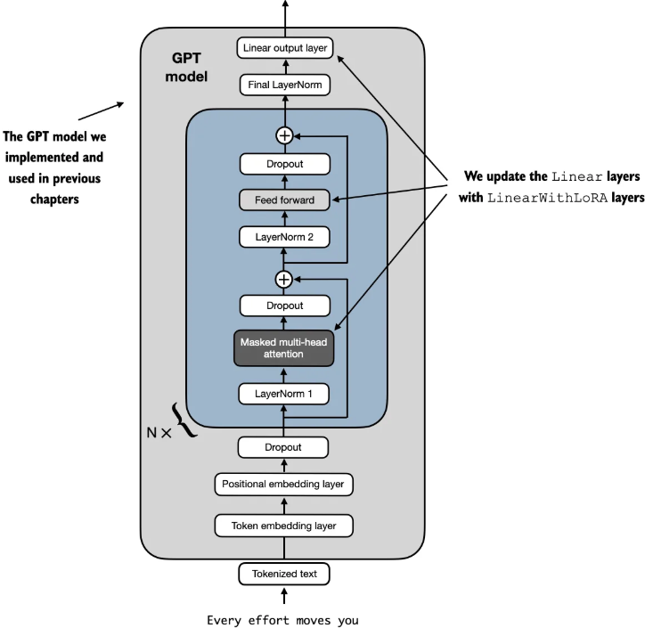
为了整合原始线性层的权重,创建一个LinearWithLoRA层。该层利用之前实现的LoRALayer,替换神经网络中现有的线性层,比如GPTModel中的自注意力模块或前馈模块

1
2
3
4
5
6
7
8
9
10
11
12
13
14
15
16
17
18
19
class LinearWithLoRA(torch.nn.Module):
''' Combine original linear layer with LoRA layer '''
def __init__(self, linear, rank, alpha):
super().__init__()
self.linear = linear
self.lora = LoRALayer(linear.in_features, linear.out_features, rank, alpha)

def forward(self, x):
# forward方法通过将原始线性层和LoRA层的结果相加来计算输出
return self.linear(x) + self.lora(x)

def replace_linear_with_lora(model, rank, alpha):
for name, module in model.named_children():
if isinstance(module, torch.nn.Linear):
# 把原来的线性层替换为LoRA层
setattr(model, name, LinearWithLoRA(module, rank, alpha))
else:
# 递归的方式替换所有层
replace_linear_with_lora(module, rank, alpha)

replace_linear_to_lora

查看替换前后的模型参数数量变化,从124,441,346减少到2,666,528。可训练参数的数量减少到了原来的1/50。将rank和alpha设置为16是一个不错的默认选择,但增加rank参数也很常见,这反过来会增加可训练参数的数量。通常选择将alpha设置为rank的一半、两倍或等于rank的值。

1
2
3
4
5
6
7
8
9
10
11
12
13
total_params = sum(p.numel() for p in model.parameters() if p.requires_grad)
print(f"Total trainable parameters before: {total_params:,}") # 124,441,346
# 把模型中所有参数设置为不训练
for param in model.parameters():
param.requires_grad = False

total_params = sum(p.numel() for p in model.parameters() if p.requires_grad)
print(f"Total trainable parameters after: {total_params:,}") # 0
# 把模型中原来的线性层替换为LoRA
replace_linear_with_lora(model, rank=16, alpha=16)

total_params = sum(p.numel() for p in model.parameters() if p.requires_grad)
print(f"Total trainable LoRA parameters: {total_params:,}") # 2,666,528

对模型微调完整流程

完整的流程这里分成了6步

1
2
3
4
5
6
7
8
9
10
11
12
13
14
15
16
17
18
19
20
21
22
23
24
25
26
27
28
29
30
31
32
33
34
35
36
37
38
39
40
41
42
43
44
45
46
47
48
49
50
51
52
53
54
55
56
57
58
59
60
61
62
63
64
65
66
67
68
69
70
71
72
73
74
75
76
77
78
def train_sms_classify_lora():
# 1. 加载数据集
# 数据集分割为3个文件,分别是训练集train.csv、验证集validtaion.csv和测试集test.csv
create_balanced_dataset()
train_loader, val_loader, test_loader = create_sms_data_loaders()

# 2. 加载预训练模型
BASE_CONFIG = {
"vocab_size": 50257, # Vocabulary size
"emb_dim": 768,
"n_layers": 12,
"n_heads": 12,
"context_length": 1024, # Context length
"drop_rate": 0.0, # Dropout rate
"qkv_bias": True # Query-key-value bias
}

settings, params = load_gpt_models(model_size='124M', models_dir="gpt2")
model = GPTModel(BASE_CONFIG)
load_weights_into_gpt(model, params)
model.eval()

# 3. 计算微调前的准确率
torch.manual_seed(123)
# set DISABLE_ADDMM_CUDA_LT=1
device = torch.device("cuda" if torch.cuda.is_available() else "cpu")
num_classes = 2 # 0表示非垃圾短信,1表示垃圾短信
# 重新定义输出层
model.out_head = torch.nn.Linear(in_features=768, out_features=num_classes)
model.to(device)

torch.manual_seed(123)
train_accuracy = calc_accuracy_loader(train_loader, model, device, num_batches=10)
val_accuracy = calc_accuracy_loader(val_loader, model, device, num_batches=10)
test_accuracy = calc_accuracy_loader(test_loader, model, device, num_batches=10)

print(f"Training accuracy: {train_accuracy*100:.2f}%") # 46.25%
print(f"Validation accuracy: {val_accuracy*100:.2f}%") # 45.00%
print(f"Test accuracy: {test_accuracy*100:.2f}%") # 48.75%

# 4. 使用LoRA微调模型
total_params = sum(p.numel() for p in model.parameters() if p.requires_grad)
print(f"Total trainable parameters before: {total_params:,}")
# 把模型中所有参数设置为不训练
for param in model.parameters():
param.requires_grad = False

total_params = sum(p.numel() for p in model.parameters() if p.requires_grad)
print(f"Total trainable parameters after: {total_params:,}")
# 把模型中原来的线性层替换为LoRA
replace_linear_with_lora(model, rank=16, alpha=16)

total_params = sum(p.numel() for p in model.parameters() if p.requires_grad)
print(f"Total trainable LoRA parameters: {total_params:,}")
# 原来的线性层被替换了,所以再把模型数据往运算设备上放一次
model.to(device)
#print(model)
start_time = time.time()
torch.manual_seed(123)
optimizer = torch.optim.AdamW(model.parameters(), lr=5e-5, weight_decay=0.1)

num_epochs = 5
train_losses, val_losses, train_accs, val_accs, examples_seen = train_classifier_simple(
model, train_loader, val_loader, optimizer, device,
num_epochs=num_epochs, eval_freq=50, eval_iter=5,
)

end_time = time.time()
execution_time_minutes = (end_time - start_time) / 60
print(f"Training completed in {execution_time_minutes:.2f} minutes.")

# 5. 评估模型
epochs_tensor = torch.linspace(0, num_epochs, len(train_losses))
examples_seen_tensor = torch.linspace(0, examples_seen, len(train_losses))
plot_values(epochs_tensor, examples_seen_tensor, train_losses, val_losses, label="loss")

# 6. 保存模型
torch.save(model.state_dict(), "review_lora_classifier.pth")

最终输出:使用的时间1.3分钟比第六章全量训练的0.68分钟还要久,可能是因为其中的矩阵乘法耗时了,生成的review_lora_classifier.pth文件大小为533M

1
2
3
4
5
6
7
8
9
10
11
12
13
14
15
16
17
18
19
20
Total trainable LoRA parameters: 2,666,528
Ep 1 (Step 000000): Train loss 3.757, Val loss 3.403
Ep 1 (Step 000050): Train loss 0.329, Val loss 0.317
Ep 1 (Step 000100): Train loss 0.170, Val loss 0.296
Training accuracy: 95.00% | Validation accuracy: 97.50%
Ep 2 (Step 000150): Train loss 0.181, Val loss 0.029
Ep 2 (Step 000200): Train loss 0.015, Val loss 0.084
Ep 2 (Step 000250): Train loss 0.045, Val loss 0.031
Training accuracy: 92.50% | Validation accuracy: 97.50%
Ep 3 (Step 000300): Train loss 0.025, Val loss 0.018
Ep 3 (Step 000350): Train loss 0.065, Val loss 0.083
Training accuracy: 100.00% | Validation accuracy: 100.00%
Ep 4 (Step 000400): Train loss 0.004, Val loss 0.046
Ep 4 (Step 000450): Train loss 0.279, Val loss 0.309
Ep 4 (Step 000500): Train loss 0.006, Val loss 0.013
Training accuracy: 100.00% | Validation accuracy: 100.00%
Ep 5 (Step 000550): Train loss 0.006, Val loss 0.001
Ep 5 (Step 000600): Train loss 0.000, Val loss 0.149
Training accuracy: 100.00% | Validation accuracy: 100.00%
Training completed in 1.30 minutes.

其中替换之后的一个transformer块内包含新的LinearWithLoRA层,这些层由设置为不可训练的原始Linear层新的LoRA层组成

1
2
3
4
5
6
7
8
9
10
11
12
13
14
15
16
17
18
19
20
21
22
23
24
25
26
27
28
29
30
31
32
33
34
35
36
37
38
39
40
41
42
GPTModel(
(tok_emb): Embedding(50257, 768)
(pos_emb): Embedding(1024, 768)
(drop_emb): Dropout(p=0.0, inplace=False)
(trf_blocks): Sequential(
(0): TransformerBlock(
(att): MultiHeadAttention(
(W_query): LinearWithLoRA(
(linear): Linear(in_features=768, out_features=768, bias=True)
(lora): LoRALayer()
)
(W_key): LinearWithLoRA(
(linear): Linear(in_features=768, out_features=768, bias=True)
(lora): LoRALayer()
)
(W_value): LinearWithLoRA(
(linear): Linear(in_features=768, out_features=768, bias=True)
(lora): LoRALayer()
)
(out_proj): LinearWithLoRA(
(linear): Linear(in_features=768, out_features=768, bias=True)
(lora): LoRALayer()
)
(dropout): Dropout(p=0.0, inplace=False)
)
(ff): FeedForward(
(layers): Sequential(
(0): LinearWithLoRA(
(linear): Linear(in_features=768, out_features=3072, bias=True)
(lora): LoRALayer()
)
(1): GELU()
(2): LinearWithLoRA(
(linear): Linear(in_features=3072, out_features=768, bias=True)
(lora): LoRALayer()
)
)
)
(norm1): LayerNorm()
(norm2): LayerNorm()
(drop_shortcut): Dropout(p=0.0, inplace=False)
)

最后的归一化层和输出层为

1
2
3
4
5
(final_norm): LayerNorm()
(out_head): LinearWithLoRA(
(linear): Linear(in_features=768, out_features=2, bias=True)
(lora): LoRALayer()
)
0%